Statistics
Basics
Testing
Null hypothesis (\(H_0\)) is the claim (conjecture) that no difference or relationship exists between two sets of data or variables being analyzed.
Alternative hypothesis (\(H_1\) or \(H_a\)) is what null hypothesis is tested against.
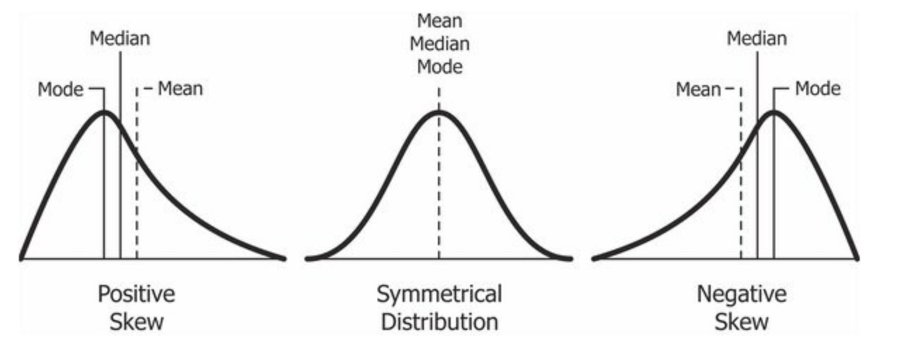
Skewness is a measure of the asymmetry of the probability distribution of a real-valued random variable about its mean.
P-value (significance) is probability that the observed pattern was created by randomness. Under the null hypothesis, the p-value is the probability of getting a sample as or more extreme than our own.
Z-score (standard score) is standard deviation.
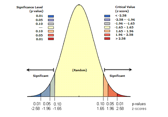
z-score (Standard Deviations) |
p-value (Probability) |
Confidence level |
|---|---|---|
< -1.65 or > +1.65 |
< 0.10 |
90% |
< -1.96 or > +1.96 |
< 0.05 |
95% |
< -2.58 or > +2.58 |
< 0.01 |
99% |
Averages
Population (arithmetic) mean/average: arithmetic average of all values in the population, defined as \(\mu = \frac{\sum_{i=1}^{n} x_i}{n}\)
Sample mean: arithmetic average of all values in a sample; an estimator of the population mean, usually denoted \(\bar{x}\).
Median: middle value when the data are ordered, such that half of the observations are below and half are above.
\[\begin{split}\tilde{x} = \begin{cases} x_{\frac{n+1}{2}}, & \text{if } n \text{ is odd} \\ \frac{x_{\frac{n}{2}} + x_{\frac{n}{2}+1}}{2}, & \text{if } n \text{ is even} \end{cases}\end{split}\]Mode is the value that appears most often in a set (there can be zero, one, or multiple modes).
Harmonic mean: appropriate for averaging rates or ratios; defined as the reciprocal of the arithmetic mean of the reciprocals of the values,
\[H = \frac{n}{\sum_{i=1}^{n} \frac{1}{x_i}}\]
Measures of dispersion (variability)
https://z-table.com/ (z-score and std_dev to left-tail probabilty)
Range: simplest measure of spread; difference between the largest and smallest values in the data.
\[R = \max_i x_i - \min_i x_i\]Variance: measures dispersion around the mean; it is the average squared deviation from the mean.
\[\begin{split}\begin{array}{cc} \sigma^2 = \frac{\sum_{i=1}^{n} (x_i - \mu)^2 }{n} & \sigma^2 = \frac{\sum_{i=1}^{n} x_i^2 }{n} - \mu^2 \\ s^2 = \frac{\sum_{i=1}^{n} (x_i - \bar{x})^2}{n-1} & s^2 = \frac{\sum_{i=1}^{n} x_i^2 - \frac{(\sum_{i=1}^{n} x_i)^2}{n} }{n-1} \end{array}\end{split}\]Standard deviation (\(\sigma\) or \(s\)): square root of the variance. It also measures dispersion, but in the same units as the data and can be interpreted as a typical distance of observations from the mean.
Z-score (standard score): standardized value that measures how many standard deviations a data point \(x\) is from the mean. For a population with mean \(\mu\) and standard deviation \(\sigma\):
\[z = \frac{x - \mu}{\sigma}\]In practice, \(\mu\) and \(\sigma\) are often replaced by the sample mean \(\bar{x}\) and sample standard deviation \(s\).
Empirical rule (68–95–99.7)
For approximately normal data (standardized as \(Z \sim N(0,1)\)):
\[P(|Z| < 1) \approx 0.68,\quad P(|Z| < 2) \approx 0.95,\quad P(|Z| < 3) \approx 0.997\]Informally: about 68%, 95%, and 99.7% of observations lie within 1, 2, and 3 standard deviations of the mean, respectively.
Counting (Combinatorics)
Let \(n\) be the total number of distinct objects.
Let \(r\) be the number of objects selected from these \(n\).
Permutations (order matters)
\({}_nP_r\) or \(P(n,r)\) denotes the number of ordered arrangements (permutations) of \(r\) objects chosen from \(n\) distinct objects.
\[{}_nP_r = P(n,r) = \frac{n!}{(n - r)!}\]
Combinations (order does not matter)
\({}_nC_r\), \(C(n,r)\) or \(\binom{n}{r}\) denotes the number of unordered selections (combinations) of \(r\) objects chosen from \(n\) distinct objects.
\[{}_nC_r = C(n,r) = \binom{n}{r} = \frac{n!}{r!\,(n - r)!}\]
Quantiles
https://en.wikipedia.org/wiki/Cumulative_distribution_function
https://pappubahry.substack.com/p/i-have-opinions-about-the-nine-definitions
Cumulative distribution function (CDF) of a real-valued random variable \(X\):
\[F_X(x) = P(X \le x), \quad x \in \mathbb{R}.\]For \(\alpha \in (0,1)\), a (lower) \(\alpha\)-quantile \(q_\alpha\) of \(X\) is defined by
\[q_\alpha = \inf\{x \in \mathbb{R} : F_X(x) \ge \alpha\}.\]If \(F_X\) is continuous and strictly increasing, the quantile is unique and satisfies
\[F_X(q_\alpha) = \alpha \quad\text{and}\quad q_\alpha = F_X^{-1}(\alpha).\]For a sample \(x_1,\dots,x_n\) with order statistics \(x_{(1)} \le \dots \le x_{(n)}\), an empirical \(\alpha\)-quantile is obtained by taking an order statistic near position \(\alpha n\) (possibly with interpolation, depending on the chosen convention).
Percentiles
The \(p\)-th percentile (for \(0 < p < 100\)) is the quantile \(q_{p/100}\); if \(F_X\) is continuous and strictly increasing, then
\[F_X\!\bigl(q_{p/100}\bigr) = \frac{p}{100}.\]Special cases (as quantiles):
Median: \(q_{0.5}\) (50th percentile).
Quartiles: \(q_{0.25} = Q_1\), \(q_{0.75} = Q_3\) (25th and 75th percentiles).
In a sample \(x_1,\dots,x_n\) with order statistics \(x_{(1)} \le \dots \le x_{(n)}\), an empirical \(p\)-th percentile is typically defined as the empirical \(q_{p/100}\) (using the empirical quantile rule chosen for the data/tool).
Percentile rank
For a finite sample \(x_1,\dots,x_n\), the percentile rank of a value \(x\) is the percentage of observations less than or equal to \(x\), e.g.
\[\mathrm{PR}(x) = 100 \cdot \frac{\#\{\,i : x_i \le x\,\}}{n},\]with minor variations in the inequality and handling of ties depending on convention.
Types of Probability
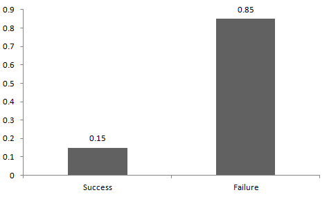
Classical (Theoretical) - Based on equally likely outcomes. - Example: P(odd on fair d6) = 3/6.
Empirical (Relative Frequency) - Based on observed data / experiments. - Example: 23 heads in 50 flips → P(heads) ≈ 23/50.
Subjective - Based on personal belief or expert judgment. - Example: Analyst estimates 60% chance of market rise.
Axiomatic - Defined via formal axioms (non-negativity, normalization, additivity). - All probability rules are derived from these.
Sampling distribution of a sample proportion
Let \(X \sim \text{Binomial}(n,p)\) be the number of “successes” in \(n\) trials. The sample proportion is
\[\hat{p} = \frac{X}{n}.\]Mean and standard deviation (standard error):
\[\mathbb{E}[\hat{p}] = p, \quad \sigma_{\hat p} = \sqrt{\frac{p(1-p)}{n}}.\]For large enough \(n\) (e.g. \(np \ge 5\) and \(n(1-p) \ge 5\)),
\[\hat{p} \approx N\!\Bigl(p,\; \frac{p(1-p)}{n}\Bigr), \quad Z = \frac{\hat{p} - p}{\sqrt{p(1-p)/n}} \approx N(0,1),\]so the empirical 68–95–99.7 rule and \(z\)-tables apply.
Standard error
Standard error (SE): the standard deviation of a statistic’s sampling distribution (i.e., how much an estimator would vary over repeated samples of the same size).
\[\mathrm{SE}(T) = \sqrt{\mathrm{Var}(T)}.\]Standard deviation vs. standard error: - SD describes variability of the data (single sample / population). - SE describes variability of an estimate (across hypothetical repeated samples).
Key scaling: for many common estimators, \(\mathrm{SE} \propto 1/\sqrt{n}\) (larger samples → smaller SE).
Common examples
Sample mean (i.i.d. with population SD \(\sigma\)):
\[\mathrm{SE}(\bar{x}) = \frac{\sigma}{\sqrt{n}}, \qquad \widehat{\mathrm{SE}}(\bar{x}) = \frac{s}{\sqrt{n}}.\]Sample proportion (\(\hat p = X/n\), \(X \sim \mathrm{Binomial}(n,p)\)):
\[\mathrm{SE}(\hat p) = \sqrt{\frac{p(1-p)}{n}}, \qquad \widehat{\mathrm{SE}}(\hat p) = \sqrt{\frac{\hat p(1-\hat p)}{n}}.\]
Use in inference (rule of thumb)
Standardized statistic often has the form
\[Z = \frac{\text{estimate} - \text{null value}}{\mathrm{SE}(\text{estimate})},\]and for large samples \(Z \approx N(0,1)\) (or a \(t\)-distribution for means when \(\sigma\) is unknown).
Types of Distributions
Discrete values
Bernoulli
Two possible outcomes (0 or 1) and a single trial.
Uniform
Poisson
Binomial
Exponential
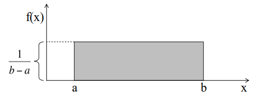
Continuous values
Normal
Kelly Criterion
Betting everything maximizes your mean wealth.
Using the Kelly Criterion maximizes your median wealth.
...
Incidentally, the choice of maximizing the median is somewhat arbitrary.
You can also use a similar approach to maximize, say, the 25th percentile outcome,
at the expense of average and median outcomes.
Causal Inference
gwern: Why Correlation Usually ≠ Causation (gwern) - gwern: Everything Is Correlated
yt: Introduction to causal inference and directed acyclic graphs (UK Reproducibility Network)
tg: Иллюстрация парадокса Берксона (Berkson’s Paradox) - Занятно, что если такое явление наблюдается при объединении маленьких выборок в большую, то это называется парадоксом Симпсона, а если маленькие выделяются из одной большой, то парадоксом Берксона - хотя суть та же. - NOTE: Я не уверен, что суть одна и так же. - Парадокс Симпсона - парадокс объединения src - Парадокс Берксона - ошибка коллайдера src
Eight basic rules for causal inference - Counter-intuitive:
Rule 8: Controlling for a causal descendant (partially) controls for the ancestor
DAGs
DAGs are directed, because causality is:
X -> Ymeans “Y listens to X” or “if we wiggle X, then Y will also wiggle”; or: changingXmodifies the probability ofY.Instead of “two-way causality” (e.g.
anxiety <--> sleep) you need to represent it as a chain of nodes causing each other (in day 1, day 2, etc).
Kinship Terminology
A -> B -> CAis a parent ofB,Bis a child ofA.AandBare ancestors ofC,Cis a descendant ofAandB.
Roles of Covariates
Variables of interest:
The exposure (independent variable; a cause).
The outcome (dependent variable).
Other variables (measured or not) are covariates.
Types of covariates:
Confounders
Mediators
Proxy confounders
Competing exposures
Path types:
Paths can be “open” (d-connected; d for “directional”) or “closed” (d-separated).
Open paths transmit associations (aka correlations or dependencies):
X -> opened -> Y.Closed paths do not transmit associations:
X -- closed -- Y.Causal path (aka directed path):
A -> C.Confounding path (aka backdoor path):
C <- A -> F. Without conditioning onA, confounding paths are open (variations inAwould appear as covariations inCandF). If we condition onA(aka clamp down onAor control/adjust for it), then we prevent that variation, and thusCandFwould no longer be associated.Collider path:
A -> F <- E. Without conditioning onF, collider paths are closed (they do not transmit dependencies betweenAandE). Conditioning onFopens the path (if we wiggleA, it will wiggleE).
Conditioning (adjusting/controlling/truncating)
Restriction
Estimating the effect in a sample with similar values of one or more other variables, e.g. non-smokers only.
Stratification
Estimating the effect in strata with similar values of one or more other variables, e.g. non-smokers, ex-smokers, current smokers.
Covariate adjustment
Estimating the effect while controlling for values of one or more other variables, e.g. including smoking as a covariate in a regression model.
Matching
Estimating the effect in clusters with similar values of one or more other variables, e.g. participants are matched on smoking status at recruitment.
Conditioning could be good (if conditioning for a confounder), or bad (if conditioning for a collider).
Causal Effect Identification
Estimand: e.g. the true difference in
Ydue to exposureX.Estimator: e.g. your regression model.
Estimate: e.g. the estimated difference in
Yfrom the model coefficient.
Estimation is different from testing:
Testing: focuses on a binary question of whether a “significant” effect is observed. Encourages bad practices (e.g. p-hacking).
Interval estimation: focuses on obtaining the most accurate estimate and uncertainty interval.
Structural Equation Modeling
SEM is a parametric DAG.
Variables
Observed: directly measured (e.g. responses to a questionnaire).
Latent: inferred from observed variables (e.g. the level of intelligence).
Endogenous: dependent variables (e.g. in
y = x1 + x2 + x3,yis the endogenous variable).Exogenous: independent variables (e.g. an athlete’s sleep time is independent of the type of racing bike).
Models
Measurement model: measures the relationships between latent constructs and observed variables. The confirmatory factor analysis framework tests the underlying hypothesis of the measurement model.
Structural model: investigates causal relationships between latent constructs. It is diagrammatically represented using path analysis.
The Only Rule of Bayesian Model
Probability of each node is conditional probability of its own given the probability of its parents.
A -> B -> C -> DP(A,B,C,D) = P(A) P(B|A) P(C|B) P(D|C)A -> C -> D,A -> B -> DP(A,B,C,D) = P(A) P(B∣A) P(C∣A) P(D∣B,C)B -> C -> D -> E,A -> DP(A,B,C,D,E) = P(A) P(B) P(C∣B) P(D∣A,C) P(E∣D)